Introduction

The Wasserstein distance and optimal transport theory were first studied by the French mathematician Gaspard Monge in the 18th entury. Since that time, the field has been revisited by many illustrious mathematicians like Leonid Kantorovich in the 20th century and more recently by the Fields medalist Cédric Villani.

In addition to these considerable theoretical advances, the method has also benefited from important advances in numerical computations and algorithms which have made it amenable to real large scale problems. Consequently, optimal transport has been applied successfully to various contexts such as regularization in statistical learning, distributionally robust optimization, image retrieval and economics.

This post focuses on the basic concepts underlying the Wasserstein distance, detailing some of its interesting properties as well as practical numerical methods. It shies away from the often math-heavy formulations and tries to focus on the important practical questions to build intuition.

Basic formalism and notation

Given an arbitrary base set Ω⊂Rd, M(Ω) denotes the set of probability measures on Ω and m(μ,ν) represents the set of joint distributions with marginals μ and ν in M(Ω). Using some distance D:Ω×Ω→R+ such as the lp norms with p∈N, the p-Wasserstein distance is then defined as the solution to the following optimization problem:

Wp(μ,ν)=infΠ∈m(μ,ν)(∫Ω∫ΩD(x,y)pdΠ(x,y))1p.

A particular, but usefull case is the situation where we consider only discrete measures. In that case, we have a finite set of points/atoms X={x1,⋯,xn} and Y={y1,⋯,ym} and the measures take the form μ=∑ni=1δxiai and ν=∑mj=1δyjbi for a∈Δn and b∈Δm where Δl={u∈Rl+:∑iui=1} is the simplex and δxi is a dirac measure putting all weight on xi.

In that case, the Wasserstein distance (to the pth power) takes on the much simpler form of a linear transportation problem, which we write explicitely in terms of the marginal probabilites a∈Δn and b∈Δm:

The problem has a simple intuitive meaning as the minimum amount of work required to transform one distribution into the other. Indeed, when p=1 this is called the Earth Mover Distance and can be though of as moving dirt from high valued bins of one distribution to throughs in another. Each time, we consider the physical distance between the bins and prioritize bins that are close to one another according to the ground distance D.

Properties and rationale

Like other distances, it is non-negative, symmetric, subadditive and 0 only if the 2 measures are identical. It also offers interesting advantages over standard distances like the Euclidean distance. For instance, we notice that n and m can be different, which implies we can compare distributions with a different number of bins.¹

Together with an adequate choice of ground distance D:Ω×Ω→R+, the Wasserstein distance can capture important local properties of the problem. Each bin of a distribution is compared to every other bin of the other distribution, but closer bins are less penalized that ones that are farther. For images, this might help capture the local correlation in pixel intensity². In contrast, using the raw Euclidean distance would require having 2 histograms with exactly the same number of bins/points/atoms and comparing values bin by bin.

As shown in the important Rubner et al. paper, these properties help the Wasserstein distance better capture perceived similarities between distributions than the standard Euclidean distance. The authors show that the Wasserstein distance remains superior even for distances induced by quadratic norms D(x,y)=||K(x−y)||2, which do not suffer from the bin by bin comparison of the standard Euclidean distance for some symmetric positive definite matrix K∈Rd×d.

A small example

Consider the following vectors x0,x1,x2∈R5, represented in the figure below:

Further assume that each of the 5 dimensions represents a position on a line so that we can determine that the distance between positions/indices 0 and 4 is D(0,4)=|0−4|, which is four times D(0,1)=|1−0|, the distance between positions 0 and 1.

Euclidean distance

As the figure on the right illustrates, all 3 vectors are all equally dissimilar with a maximal Euclidean distance of √2 since they differ by 1 at exactly 2 positions. Hence the normalized distance is 1 off the diagonal and 0 otherwise.

Wasserstein distance

The figure below illustrates that the result is different when computing the Wasserstein distance between the 3 discrete measures μi=δji,i=0,⋯,2 placing unit mass at j0=0,j1=1,j2=4. Indeed, with that choice of distance, x0 and x1 are much closer than x0 and x2 and x1 and x2³.

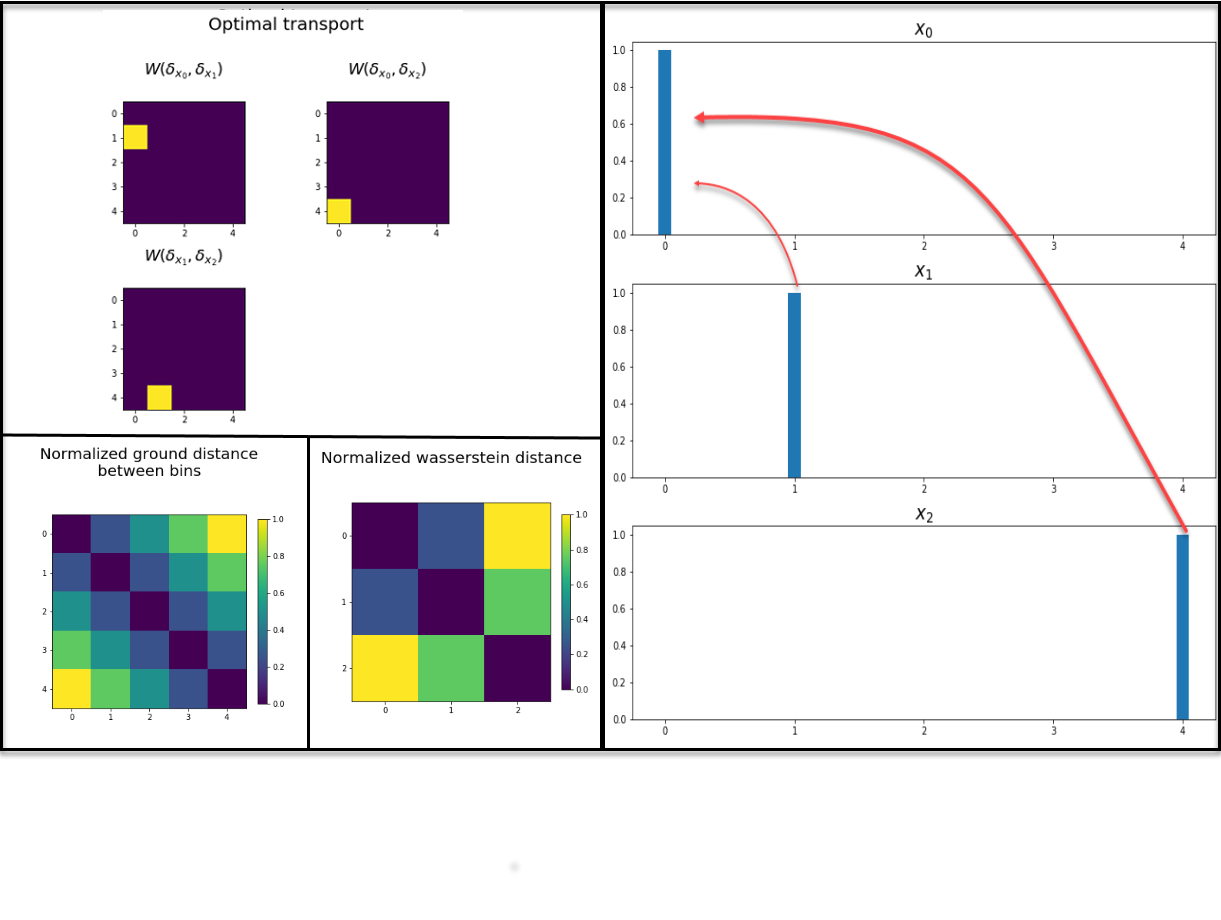
Computing the Wasserstein distance between three discrete measures with a single atom. Although the ground distance is symmetric accross both diagonals, the Wasserstein distance reflects the intuitive fact that moving 1 unit of mass from 4 to 1 is costlier than moving it from 4 to 0. The top left and right quadrants illustrate the optimal transport plan while the central bottom square illustrates the actual normalized Wasserstein distance.

Wasserstein barycenters

It is also interesting to study the barycenters generated by the Wasserstein distance. Following our intuition based on the usual Euclidean norm and the fact that ∑Ni=1xiN∈argmaxu∑Ni=11N||xi−u||2 (which is one of the key results underlying the k-means algorithm for instance), we can think of barycenters as centroids or representative of a set of objects (measures in this case). More formally, given a set of N distributions {νi}Ni=1, the Wasserstein barycenter is defined as the measure that minimizes the following problem:

μ∗=argminμ1NN∑i=1Wpp(μ,νi)

The following sections detail two important cases in which we can find such solutions either numerically or analytically.

Analytical solution for Gaussian distributions

In the specific case where νi∼N(mi,Σi) are all Gaussian, Agueh and Carlier show that μ∗∼N(∑Ni=1miN,ˆΣ), where ˆΣ is a semidefinite symmetric matrix satisfying ˆΣ=1N∑Ni=1(ˆΣ1/2ΣiˆΣ1/2)1/2. In other words, the barycenter remains Gaussian with a mean given by the arithmetic average of the mean of the {νi} and the covariance matrix satisfies a non-linear equation.

As illustrated in the figure below, this contrasts with the mixture distribution ∑Ni=11NN(mi,Σi) which is in general not Gaussian. This shape preserving property has numerous useful applications in image processing, particularly for texture interpolation and texture mixing.

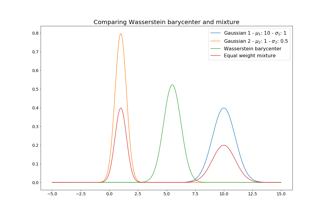
Comparing Wasserstein barycenter and mixture for Gaussian distributions.

The Wasserstein barycenter in the preceding example was computed using the excellent ot Python module. For more details and in-depth examples, check out the documentation.

Conclusion

This post illustrates that the Wasserstein distance is an extremelly powerful and versatile concept. Its locally aware shape preserving properties can be used for numerous applications and it benefits from various sophisticated numerical algorithms.

Regardless of these important advances, the field of optimal transport theory is extremelly rich and dynamic. As of 2020, many theoretical and practical research initiatives are underway and numerous applications are still being developped.